Fitting single flow curve

This notebook contains a list scripts focusing on analysis and visualization of a single flow curve. A flow curve is the measurement of the viscosity as a function of shear rate. In a measurment a constant shear rate is imposed on a fluid sample and the required shear stress is measured.

Since for Non newtonian fluids the viscosity is a function of the shear rate, the flow curve measurement is a way to characterize such functional dependence.

Rheological models can be used to fit the flow curve and extract parameters that in some case directly relates to fundamental material properties.

In this notebook we provide some example of analysis of flow curves using powerful python libraries that we simply integrate to make flow curves analysis simple, easy to share and reproduce.

We provide a sequence of exaples structured as “recepies” each with a specific scope, plotting data, fitting data, evaluating confidence itervals…

Each recepy can be considered “stand alone” meaning that the only objects that cells share are the general imports in the first cell and the functions defined through the notebook. This should make it easy to copy and paste a cell in case you want to use it as a starting point for your own analysis.

If you have a google account you can run this documentation notebook Open in colab

#executing the notebook in colab requires installation of the rheofit library
!pip install git+https://github.com/marcocaggioni/rheofit.git

%matplotlib inline

import sys
sys.path.append("./../") #in case you are running the notebook in binder or from the cloned repository
import rheofit
import lmfit
import pybroom as pb
import matplotlib.pyplot as plt
import pandas as pd
import emcee
import corner
import seaborn

Getting Example flow curve data

To make demonstration simple we stored an example flow curve in the rheodata module. In the future we would like to collect flow curves from published works to make them easily available for training purpouse.

The data provided refer to a 75w% mineral oil in 11%LAS surfactant solution. The emusion droplets size ranges from 1-10 um and the measurement was performed with a Couette geometry at 40C.

The example_emulsion method returns a Pandas dataframe with column ‘Shear rate’ in [1/s] and column ‘Stress’ in [Pa]. The choice of the name convention is from the excel exported file by the TA Trios software. A possibly better choice could be the RheoML convention ‘ShearRate’ and ‘ShearStress’.

Example of importing data from different file formats are provided in a different Notebook, here we focus on possible analysis and visualization on a single flow curve.

#using provided example data
example_data=rheofit.rheodata.example_emulsion()
example_data.head()

	Shear rate	Stress
0	999.89475	131.22475
1	891.25100	121.57225
2	794.32825	112.56525
3	707.94600	104.25800
4	630.95750	96.58295

Plotting flow curve data

To plot the data we use matplolib. We define a simple function that plot the data, set x and y scale to log and the label for x and y. The function return a matplolib figure object that can be stored in a variable.

data=rheofit.rheodata.example_emulsion()

def plot_data(data):
    plt.plot(data['Shear rate'],data['Stress'],'o')
    plt.yscale('log')
    plt.xscale('log')
    plt.ylabel('$\sigma [Pa]$');
    plt.xlabel('$\dot\gamma [1/s]$');

    return plt.gcf()

fig1=plot_data(data);

Fitting flow curve data to a rheological model

This is the most important functionality mostly provided by the LMFIT library. The rheofit module just provide the rheology model definition and documentation.

For example a popular model for yield stress fluids is the Hershel Bulckley model is a lmfit.Model object

rheofit.models.HB_model

<lmfit.Model: Model(HB, prefix='HB_')>

The model object is based on the function rheofit.models.HB

help(rheofit.models.HB)

Help on function HB in module rheofit.models:

HB(x, ystress=1.0, K=1.0, n=0.5)
    Hershel-Bulkley Model

    Note:

    .. math::
       \sigma= \sigma_y + K \cdot \dot\gamma^n

    Args:
        ystress: yield stress [Pa]

        K : Consistency index [Pa s^n]

        n : Shear thinning index []

    Returns:
        stress : Shear Stress, [Pa]

To fit the data we use the fit method of the model object passing the stress, the shear rate and the weights

data=rheofit.rheodata.example_emulsion()
model=rheofit.models.HB_model
res_fit=model.fit(data['Stress'],x=data['Shear rate'],weights=1/(data['Stress']))
res_fit

Model

Model(HB, prefix='HB_')

Fit Statistics

fitting method	leastsq
# function evals	29
# data points	101
# variables	3
chi-square	0.52363806
reduced chi-square	0.00534325
Akaike info crit.	-525.469582
Bayesian info crit.	-517.624221

Variables

name	value	standard error	relative error	initial value	min	max	vary
HB_ystress	3.18629490	0.06296913	(1.98%)	1.0	0.00000000	inf	True
HB_K	2.56281495	0.09118889	(3.56%)	1.0	0.00000000	inf	True
HB_n	0.53928815	0.00752288	(1.39%)	0.5	0.00000000	1.00000000	True

Correlations (unreported correlations are < 0.100)

HB_K	HB_n	-0.9380
HB_ystress	HB_K	-0.7366
HB_ystress	HB_n	0.6757

Plotting Fit results

The fit method returns a fit result object that contains all the information on the data, the model used and the results

data=rheofit.rheodata.example_emulsion()
data=data[data['Shear rate']>0.1]
model=rheofit.models.HB_model
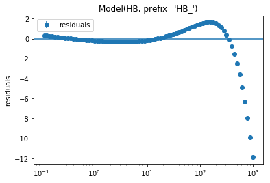
res_fit=model.fit(data['Stress'],x=data['Shear rate'],weights=1/(data['Stress']*0.1))

kwarg={'xscale':'log','yscale':('log')}
res_fit.plot_fit(ax_kws=kwarg,yerr=False);
plt.figure()
res_fit.plot_residuals(yerr=False,ax_kws={'xscale':'log'})

<matplotlib.axes._subplots.AxesSubplot at 0x7fed09a0c8d0>

data=rheofit.rheodata.example_emulsion()
data=data[data['Shear rate']>0.1]

model=rheofit.models.HB_model
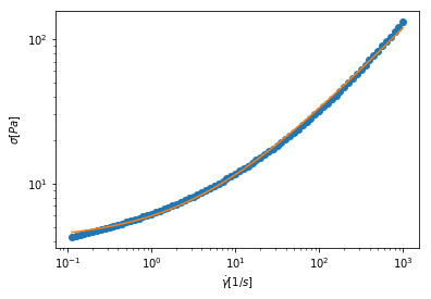
res_fit=model.fit(data['Stress'],x=data['Shear rate'],weights=1/(data['Stress']))

def plot_fit(res_fit, xlist=None):
    if xlist is None:
        xlist=res_fit.userkws['x']

    plt.plot(res_fit.userkws['x'], res_fit.data,'o',label='Data')
    plt.plot(xlist, res_fit.eval(x=xlist),label='Best fit')
    plt.yscale('log')
    plt.xscale('log')
    plt.ylabel('$\sigma [Pa]$')
    plt.xlabel('$\dot\gamma [1/s]$')

plot_fit(res_fit);

Explore fit results with pybroom

Exploring the lmfit.fit_result object is not intuitive, using the convenient pybroom library make things very easy, especially when we explore lists of results from different sample.

data=rheofit.rheodata.example_emulsion()
model=rheofit.models.HB_model
res_fit=model.fit(data['Stress'],x=data['Shear rate'],weights=1/(data['Stress']))

pb.glance(res_fit)

	model	method	num_params	num_data_points	chisqr	redchi	AIC	BIC	num_func_eval	success	message
0	Model(HB, prefix='HB_')	leastsq	3	101	0.523638	0.005343	-525.469582	-517.624221	29	True	Fit succeeded.

data=rheofit.rheodata.example_emulsion()
model=rheofit.models.HB_model
res_fit=model.fit(data['Stress'],x=data['Shear rate'],weights=1/(data['Stress']))

pb.tidy(res_fit)

	name	value	min	max	vary	expr	stderr	init_value
0	HB_K	2.562815	0	inf	True	NaN	0.091189	1.0
1	HB_n	0.539288	0	1.0	True	NaN	0.007523	0.5
2	HB_ystress	3.186295	0	inf	True	NaN	0.062969	1.0

data=rheofit.rheodata.example_emulsion()
model=rheofit.models.HB_model
res_fit=model.fit(data['Stress'],x=data['Shear rate'],weights=1/(data['Stress']))

augmented=pb.augment(res_fit)
augmented.head()

	x	data	best_fit	residual
0	999.89475	131.22475	109.492113	-0.165614
1	891.25100	121.57225	103.098212	-0.151959
2	794.32825	112.56525	97.083545	-0.137535
3	707.94600	104.25800	91.430975	-0.123032
4	630.95750	96.58295	86.118672	-0.108345

Plot residuals

data=rheofit.rheodata.example_emulsion()
model=rheofit.models.HB_model
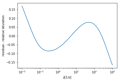
res_fit=model.fit(data['Stress'],x=data['Shear rate'],weights=1/(data['Stress']))


def plot_residuals(res_fit):
    augmented=pb.augment(res_fit)
    plt.plot('x','residual',data=augmented)
    plt.xscale('log')
    plt.ylabel('residual - relative deviation');
    plt.xlabel('$\dot\gamma [1/s]$');

    return plt.gcf()

plot_residuals(res_fit);

Confidence interval

data=rheofit.rheodata.example_emulsion()
data=data[data['Shear rate']>0.1]
model=rheofit.models.HB_model
res_fit=model.fit(data['Stress'],x=data['Shear rate'],weights=1/(data['Stress']))

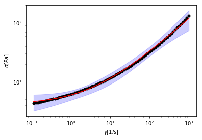
def plot_confidence(res_fit,expand=10):
    dely = res_fit.eval_uncertainty(x=res_fit.userkws['x'],sigma=3)*expand

    plt.plot(res_fit.userkws['x'], res_fit.data,'o',color='black',label='Data',markersize=5)
    plt.plot(res_fit.userkws['x'], res_fit.best_fit,label='Best fit TC model',color='red')
    plt.fill_between(res_fit.userkws['x'], res_fit.best_fit-dely,res_fit.best_fit+dely,
                     color='blue',alpha=0.2,label='0.9973 Confidence interval')
    plt.yscale('log')
    plt.xscale('log')
    plt.ylabel('$\sigma [Pa]$')
    plt.xlabel('$\dot\gamma [1/s]$')

    return plt.gcf()

plot_confidence(res_fit);

Fit specific shear rate range

data=rheofit.rheodata.example_emulsion()
data=data[data['Shear rate']>0.1]
model=rheofit.models.HB_model
res_fit=model.fit(data['Stress'],x=data['Shear rate'],weights=1/(data['Stress']))

min_shear_rate=0.1
max_shear_rate=1000

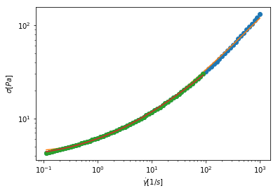
def fit_range(res_fit,min_shear_rate=0.1,max_shear_rate=100):
    data=pd.DataFrame.from_dict({'Shear rate':res_fit.userkws['x'],'Stress':res_fit.data})
    mask=(data['Shear rate']>=min_shear_rate) & (data['Shear rate']<=max_shear_rate)
    res_fit=model.fit(data[mask]['Stress'],x=data[mask]['Shear rate'],weights=1/(data[mask]['Stress']))

    return res_fit

plot_fit(res_fit);
plot_fit(fit_range(res_fit));

data=rheofit.rheodata.example_emulsion()
model=rheofit.models.HB_model
res_fit=model.fit(data['Stress'],x=data['Shear rate'],weights=1/(data['Stress']))

min_shear_rate=0.1
max_shear_rate=1000

def fit_range(res_fit,min_shear_rate=0.1,max_shear_rate=100):
    data=pd.DataFrame.from_dict({'Shear rate':res_fit.userkws['x'],'Stress':res_fit.data})
    mask=(data['Shear rate']>min_shear_rate) & (data['Shear rate']<max_shear_rate)
    res_fit=model.fit(data[mask]['Stress'],x=data[mask]['Shear rate'],weights=1/(data[mask]['Stress']))

    return res_fit

display(pb.tidy(fit_range(res_fit,min_shear_rate=0.1,max_shear_rate=10)))
display(pb.tidy(fit_range(res_fit,min_shear_rate=0.1,max_shear_rate=100)))
display(pb.tidy(fit_range(res_fit,min_shear_rate=0.1,max_shear_rate=1000)))

	name	value	min	max	vary	expr	stderr	init_value
0	HB_K	2.946032	0	inf	True	NaN	0.033507	1.0
1	HB_n	0.452852	0	1.0	True	NaN	0.004298	0.5
2	HB_ystress	3.219395	0	inf	True	NaN	0.028909	1.0

	name	value	min	max	vary	expr	stderr	init_value
0	HB_K	2.498040	0	inf	True	NaN	0.037762	1.0
1	HB_n	0.517414	0	1.0	True	NaN	0.003954	0.5
2	HB_ystress	3.589250	0	inf	True	NaN	0.034026	1.0

	name	value	min	max	vary	expr	stderr	init_value
0	HB_K	1.880492	0	inf	True	NaN	0.051488	1.0
1	HB_n	0.595807	0	1.0	True	NaN	0.005270	0.5
2	HB_ystress	4.088222	0	inf	True	NaN	0.059816	1.0

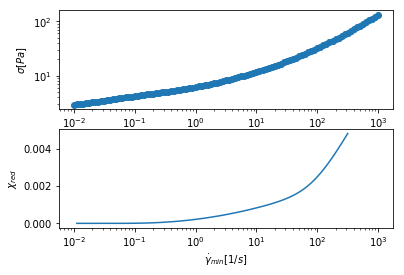
Reduced \(\chi^2\) sensitivity on shear rate range

data=rheofit.rheodata.example_emulsion()
model=rheofit.models.HB_model
res_fit=model.fit(data['Stress'],x=data['Shear rate'],weights=1/(data['Stress']))


def explore_redchi(res_fit,min_shear_rate=0.01,max_shear_rate=1000):
    data=pd.DataFrame.from_dict({'Shear rate':res_fit.userkws['x'],'Stress':res_fit.data})
    res_dict={min_shear:fit_range(res_fit,min_shear_rate=min_shear,max_shear_rate=1000)
              for min_shear in data['Shear rate'][10:-1]}

    ax1= plt.subplot(2,1,1)

    plt.plot(data['Shear rate'],data['Stress'],'o')
    plt.yscale('log')
    plt.xscale('log')
    plt.xlabel('$\dot\gamma [1/s]$')
    plt.ylabel('$\sigma [Pa]$')

    ax2= plt.subplot(2,1,2,sharex = ax1)

    plt.plot(list(res_dict.keys()),pb.glance(res_dict)['redchi'])
    plt.xscale('log')
    plt.ylabel('$\chi_{red}$')
    plt.xlabel('$\dot\gamma_{min} [1/s]$')

    return plt.gcf()

explore_redchi(res_fit);

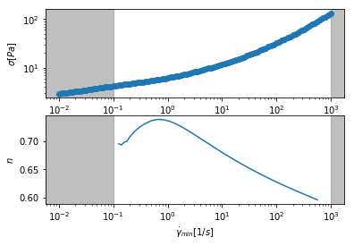
Model parameter sensitivity on shear rate range

data=rheofit.rheodata.example_emulsion()
data.sort_values('Shear rate',ascending=False, inplace=True)

model=rheofit.models.HB_model
res_fit=model.fit(data['Stress'],x=data['Shear rate'],weights=1/(data['Stress']))


def explore_param_keephigh(res_fit,min_shear_rate=0.01,max_shear_rate=1000,param_name=None):
    '''keep the right range of data for the fit
    answer the question: how important it is how low we extend the analysis at low shear?
    '''
    data=pd.DataFrame.from_dict({'Shear rate':res_fit.userkws['x'],'Stress':res_fit.data})
    data.sort_values('Shear rate',ascending=False, inplace=True)
    res_fit=res_fit.model.fit(data['Stress'],x=data['Shear rate'],weights=1/(data['Stress']))
    res_fit=fit_range(res_fit,min_shear_rate=min_shear_rate,max_shear_rate=max_shear_rate)
    res_dict={min_shear:fit_range(res_fit,min_shear_rate=min_shear,max_shear_rate=max(res_fit.userkws['x']))
              for min_shear in res_fit.userkws['x'][5:-1]}

    ax1= plt.subplot(2,1,1)

    plt.plot(data['Shear rate'],data['Stress'],'o')
    plt.yscale('log')
    plt.xscale('log')
    plt.xlabel('$\dot\gamma [1/s]$')
    plt.ylabel('$\sigma [Pa]$')

    xlim=plt.gca().get_xlim()
    plt.axvspan(xlim[0],min_shear_rate,color='gray',alpha=0.5)
    plt.axvspan(max_shear_rate,xlim[1],color='gray',alpha=0.5)

    ax2= plt.subplot(2,1,2,sharex = ax1)

    plt.plot(list(res_dict.keys()),pb.tidy(res_dict)['value'][pb.tidy(res_dict)['name']=='HB_n'])
    plt.xscale('log')
    plt.ylabel('$'+param_name+'$')
    plt.xlabel('$\dot\gamma_{min} [1/s]$')

    plt.axvspan(xlim[0],min_shear_rate,color='gray',alpha=0.5)
    plt.axvspan(max_shear_rate,xlim[1],color='gray',alpha=0.5)

    plt.gca().set_xlim(xlim)

    return plt.gcf()

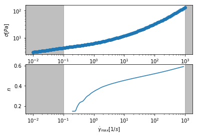
explore_param_keephigh(res_fit,min_shear_rate=0.1,param_name='n');

data=rheofit.rheodata.example_emulsion()
data.sort_values('Shear rate',ascending=False, inplace=True)

model=rheofit.models.HB_model
res_fit=model.fit(data['Stress'],x=data['Shear rate'],weights=1/(data['Stress']))


def explore_param_keeplow(res_fit,min_shear_rate=0.01,max_shear_rate=1001,param_name=None):
    '''keep the right range of data for the fit
    answer the question: how important it is how low we extend the analysis at low shear?
    '''

    data=pd.DataFrame.from_dict({'Shear rate':res_fit.userkws['x'],'Stress':res_fit.data})
    data.sort_values('Shear rate',ascending=True, inplace=True)
    res_fit=res_fit.model.fit(data['Stress'],x=data['Shear rate'],weights=1/(data['Stress']))
    res_fit=fit_range(res_fit,min_shear_rate=min_shear_rate,max_shear_rate=max_shear_rate)
    res_dict={max_shear:fit_range(res_fit,min_shear_rate=min(res_fit.userkws['x']),max_shear_rate=max_shear)
              for max_shear in res_fit.userkws['x'][5:-1]}

    ax1= plt.subplot(2,1,1)

    plt.plot(data['Shear rate'],data['Stress'],'o')
    plt.yscale('log')
    plt.xscale('log')
    plt.xlabel('$\dot\gamma [1/s]$')
    plt.ylabel('$\sigma [Pa]$')

    xlim=plt.gca().get_xlim()
    plt.axvspan(xlim[0],min_shear_rate,color='gray',alpha=0.5)
    plt.axvspan(max_shear_rate,xlim[1],color='gray',alpha=0.5)

    ax2= plt.subplot(2,1,2,sharex = ax1)

    plt.plot(list(res_dict.keys()),pb.tidy(res_dict)['value'][pb.tidy(res_dict)['name']=='HB_n'])
    plt.xscale('log')
    plt.ylabel('$'+param_name+'$')
    plt.xlabel('$\dot\gamma_{max} [1/s]$')

    plt.axvspan(xlim[0],min_shear_rate,color='gray',alpha=0.5)
    plt.axvspan(max_shear_rate,xlim[1],color='gray',alpha=0.5)

    plt.gca().set_xlim(xlim)

    return plt.gcf()

explore_param_keeplow(res_fit,min_shear_rate=0.1,param_name='n');

Emcee

data=rheofit.rheodata.example_emulsion()
data=data[data['Shear rate']>0.1]
model=rheofit.models.HB_model
res_fit=model.fit(data['Stress'],x=data['Shear rate'],weights=1/(data['Stress']*0.1))
res_emcee=res_fit.emcee(steps=1000, nwalkers=50, burn=300)

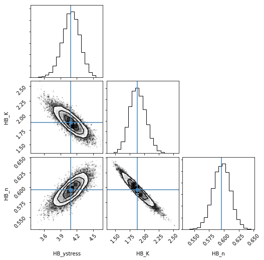
corner.corner(res_emcee.flatchain, labels=res_emcee.var_names, truths=[res_fit.params[key].value for key in res_fit.params.keys()]);
display(res_fit)

/usr/local/lib/python3.6/dist-packages/emcee/ensemble.py:258: RuntimeWarning: Initial state is not linearly independent and it will not allow a full exploration of parameter space
  category=RuntimeWarning,
100%|██████████| 1000/1000 [01:23<00:00, 12.12it/s]

Model

Model(HB, prefix='HB_')

Fit Statistics

fitting method	leastsq
# function evals	22
# data points	80
# variables	3
chi-square	10.8588639
reduced chi-square	0.14102421
Akaike info crit.	-153.763595
Bayesian info crit.	-146.617515

Variables

name	value	standard error	relative error	initial value	min	max	vary
HB_ystress	4.08822217	0.05981584	(1.46%)	1.0	0.00000000	inf	True
HB_K	1.88049246	0.05148762	(2.74%)	1.0	0.00000000	inf	True
HB_n	0.59580716	0.00527012	(0.88%)	0.5	0.00000000	1.00000000	True

Correlations (unreported correlations are < 0.100)

HB_K	HB_n	-0.9655
HB_ystress	HB_K	-0.8080
HB_ystress	HB_n	0.7536