Quickstart guide
If you have a google account you can run this documentation notebook Open in colab
[ ]:
!pip install git+https://github.com/marcocaggioni/rheofit.git
[1]:
import rheofit
import numpy as np
import pandas as pd
import pybroom as pb
import matplotlib.pyplot as plt
import seaborn as sns
sns.set_style('whitegrid')
Creating a few test datasets.
In real life you will need to import the data from a csv or excel file. Pandas is a good choice to do that.
Here we are generating artificial data and making two colums dataframes.
The two colums are ‘Shear rate’ from 0.001 1/s to 1000 1/s and stress calculated with different yield stress fluid models.
I also stick a label as a property to the dataframe to carry with me information about which sample the data belong to. I could add a third column with the label, in a tidy way, but I cannot yet convince myself it is better.
[2]:
test_data_bingham=pd.DataFrame.from_dict({'Shear rate':np.logspace(-3,3),'Stress':rheofit.models.Bingham(np.logspace(-3,3),ystress=1,eta_bg=0.1)})
test_data_bingham.label='test_data_bingham'

test_data_HB=pd.DataFrame.from_dict({'Shear rate':np.logspace(-3,3),'Stress':rheofit.models.HB(np.logspace(-3,3),ystress=1,K=1,n=0.6)})
test_data_HB.label='test_data_HB'

test_data_casson=pd.DataFrame.from_dict({'Shear rate':np.logspace(-3,3),'Stress':rheofit.models.casson(np.logspace(-3,3),ystress=1,eta_bg=0.1)})
test_data_casson.label='test_data_casson'

display(test_data_bingham.head())
| Shear rate | Stress | |
|---|---|---|
| 0 | 0.001000 | 1.000100 |
| 1 | 0.001326 | 1.000133 |
| 2 | 0.001758 | 1.000176 |
| 3 | 0.002330 | 1.000233 |
| 4 | 0.003089 | 1.000309 |
[3]:
#make a list with all the data
data_list=[test_data_bingham,test_data_casson,test_data_HB]
[4]:
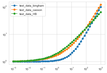
# look at the data
for data in data_list:
  plt.loglog('Shear rate','Stress',data=data,marker='o',label=data.label)
  plt.legend()
[6]:
#select a model
model=rheofit.models.HB_model
#make a list of fit_result
res_fit_dict={data.label:model.fit(data['Stress'],x=data['Shear rate']) for data in data_list}
[7]:
pb.glance(res_fit_dict)
[7]:
| model | method | num_params | num_data_points | chisqr | redchi | AIC | BIC | num_func_eval | success | message | key | |
|---|---|---|---|---|---|---|---|---|---|---|---|---|
| 0 | Model(HB, prefix='HB_') | leastsq | 3 | 50 | 9.804082e-26 | 2.085975e-27 | -3068.821831 | -3063.085762 | 131 | True | Fit succeeded. | test_data_bingham |
| 1 | Model(HB, prefix='HB_') | leastsq | 3 | 50 | 8.055381e+00 | 1.713911e-01 | -85.284137 | -79.548068 | 47 | True | Fit succeeded. | test_data_casson |
| 2 | Model(HB, prefix='HB_') | leastsq | 3 | 50 | 1.627075e-27 | 3.461862e-29 | -3273.751832 | -3268.015763 | 25 | True | Fit succeeded. | test_data_HB |
[8]:
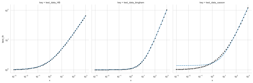
augmented_table = pb.augment(res_fit_dict)
grid = sns.FacetGrid(augmented_table, col="key", col_wrap=3,height=5)
grid.map(plt.plot, 'x', 'data', marker='o', ls='None', ms=3, color='k').set(yscale = 'log').set(xscale = 'log')
grid.map(plt.plot, 'x', 'best_fit', ls='--')
[8]:
<seaborn.axisgrid.FacetGrid at 0x1e54d7c8b88>
[9]:
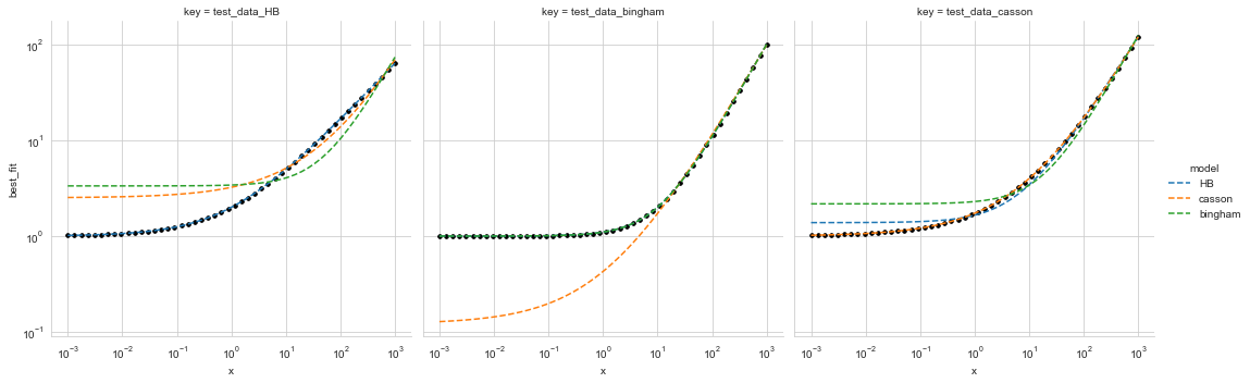
# or I can try different models
res_fit_dict_HB={data.label:rheofit.models.HB_model.fit(data['Stress'],x=data['Shear rate']) for data in data_list}
res_fit_dict_casson={data.label:rheofit.models.casson_model.fit(data['Stress'],x=data['Shear rate']) for data in data_list}
res_fit_dict_bingham={data.label:rheofit.models.Bingham_model.fit(data['Stress'],x=data['Shear rate']) for data in data_list}

augmented_table_HB=pb.augment(res_fit_dict_HB)
augmented_table_HB['model']='HB'
augmented_table_casson=pb.augment(res_fit_dict_casson)
augmented_table_casson['model']='casson'
augmented_table_bingham=pb.augment(res_fit_dict_bingham)
augmented_table_bingham['model']='bingham'

augmented_table_full=pd.concat([augmented_table_HB,augmented_table_casson,augmented_table_bingham],sort=False)
[10]:
grid = sns.FacetGrid(augmented_table_full, col="key", hue='model', col_wrap=3,height=5)
grid.map(plt.plot, 'x', 'data', marker='o', ls='None', ms=3, color='k').set(yscale = 'log').set(xscale = 'log')
grid.map(plt.plot, 'x', 'best_fit', ls='--').add_legend()
[10]:
<seaborn.axisgrid.FacetGrid at 0x1e54e3014c8>
[11]:
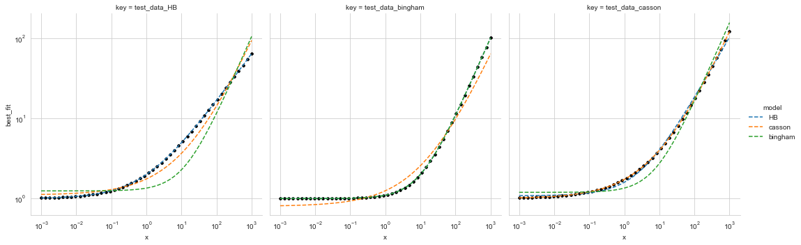
#I may want to try to pass weight to the fit since I prefer to minimize the relative deviation from the data
res_fit_dict_HB={data.label:rheofit.models.HB_model.fit(data['Stress'],x=data['Shear rate'],weights=1/data['Stress']) for data in data_list}
res_fit_dict_casson={data.label:rheofit.models.casson_model.fit(data['Stress'],x=data['Shear rate'],weights=1/data['Stress']) for data in data_list}
res_fit_dict_bingham={data.label:rheofit.models.Bingham_model.fit(data['Stress'],x=data['Shear rate'],weights=1/data['Stress']) for data in data_list}

augmented_table_HB=pb.augment(res_fit_dict_HB)
augmented_table_HB['model']='HB'
augmented_table_casson=pb.augment(res_fit_dict_casson)
augmented_table_casson['model']='casson'
augmented_table_bingham=pb.augment(res_fit_dict_bingham)
augmented_table_bingham['model']='bingham'

augmented_table_full=pd.concat([augmented_table_HB,augmented_table_casson,augmented_table_bingham],sort=False)
[12]:
grid = sns.FacetGrid(augmented_table_full, col="key", hue='model', col_wrap=3,height=5)
grid.map(plt.plot, 'x', 'data', marker='o', ls='None', ms=3, color='k').set(yscale = 'log').set(xscale = 'log')
grid.map(plt.plot, 'x', 'best_fit', ls='--').add_legend()
[12]:
<seaborn.axisgrid.FacetGrid at 0x1e54ed89688>
[13]:
#finally I want to create a table with all my result
HB_table=pb.tidy(res_fit_dict_HB)
casson_table=pb.tidy(res_fit_dict_casson)
bingham_table=pb.tidy(res_fit_dict_bingham)

full_table=pd.concat([HB_table,casson_table,bingham_table])
full_table
[13]:
| name | value | min | max | vary | expr | stderr | init_value | key | |
|---|---|---|---|---|---|---|---|---|---|
| 0 | HB_K | 0.100000 | 0 | inf | True | NaN | 7.252354e-16 | 1.0 | test_data_bingham |
| 1 | HB_n | 1.000000 | 0 | 1.0 | True | NaN | 7.094487e-16 | 0.5 | test_data_bingham |
| 2 | HB_ystress | 1.000000 | 0 | inf | True | NaN | 1.400365e-15 | 1.0 | test_data_bingham |
| 3 | HB_K | 0.506446 | 0 | inf | True | NaN | 2.153864e-02 | 1.0 | test_data_casson |
| 4 | HB_n | 0.768100 | 0 | 1.0 | True | NaN | 9.126069e-03 | 0.5 | test_data_casson |
| 5 | HB_ystress | 1.085333 | 0 | inf | True | NaN | 1.488802e-02 | 1.0 | test_data_casson |
| 6 | HB_K | 1.000000 | 0 | inf | True | NaN | 0.000000e+00 | 1.0 | test_data_HB |
| 7 | HB_n | 0.600000 | 0 | 1.0 | True | NaN | 0.000000e+00 | 0.5 | test_data_HB |
| 8 | HB_ystress | 1.000000 | 0 | inf | True | NaN | 0.000000e+00 | 1.0 | test_data_HB |
| 0 | casson_eta_bg | 0.050126 | 0 | inf | True | NaN | 4.049998e-03 | 0.1 | test_data_bingham |
| 1 | casson_ystress | 0.799855 | 0 | inf | True | NaN | 3.563013e-02 | 1.0 | test_data_bingham |
| 2 | casson_eta_bg | 0.100000 | 0 | inf | True | NaN | 1.298360e-17 | 0.1 | test_data_casson |
| 3 | casson_ystress | 1.000000 | 0 | inf | True | NaN | 8.407098e-17 | 1.0 | test_data_casson |
| 4 | casson_eta_bg | 0.074314 | 0 | inf | True | NaN | 4.212753e-03 | 0.1 | test_data_HB |
| 5 | casson_ystress | 1.105653 | 0 | inf | True | NaN | 3.785665e-02 | 1.0 | test_data_HB |
| 0 | bingham_eta_bg | 0.100000 | 0 | inf | True | NaN | 1.248824e-17 | 0.1 | test_data_bingham |
| 1 | bingham_ystress | 1.000000 | 0 | inf | True | NaN | 8.383151e-17 | 1.0 | test_data_bingham |
| 2 | bingham_eta_bg | 0.154790 | 0 | inf | True | NaN | 7.723031e-03 | 0.1 | test_data_casson |
| 3 | bingham_ystress | 1.194001 | 0 | inf | True | NaN | 4.254396e-02 | 1.0 | test_data_casson |
| 4 | bingham_eta_bg | 0.103764 | 0 | inf | True | NaN | 9.787045e-03 | 0.1 | test_data_HB |
| 5 | bingham_ystress | 1.244297 | 0 | inf | True | NaN | 7.553687e-02 | 1.0 | test_data_HB |
[ ]:
# and save it to a file
full_table.to_excel('fit_parameter_table.xls')
[93]:
pd.read_excel('fit_parameter_table.xls')
[93]:
| Unnamed: 0 | name | value | min | max | vary | expr | stderr | init_value | key | |
|---|---|---|---|---|---|---|---|---|---|---|
| 0 | 0 | HB_K | 1.000000 | 0 | inf | True | NaN | 1.304959e-16 | 1.0 | test_data_HB |
| 1 | 1 | HB_n | 0.600000 | 0 | 1.0 | True | NaN | 2.829384e-17 | 0.5 | test_data_HB |
| 2 | 2 | HB_ystress | 1.000000 | 0 | inf | True | NaN | 6.536236e-17 | 1.0 | test_data_HB |
| 3 | 3 | HB_K | 0.100000 | 0 | inf | True | NaN | 7.037382e-16 | 1.0 | test_data_bingham |
| 4 | 4 | HB_n | 1.000000 | 0 | 1.0 | True | NaN | 6.803276e-16 | 0.5 | test_data_bingham |
| 5 | 5 | HB_ystress | 1.000000 | 0 | inf | True | NaN | 1.343320e-15 | 1.0 | test_data_bingham |
| 6 | 6 | HB_K | 0.506446 | 0 | inf | True | NaN | 2.153864e-02 | 1.0 | test_data_casson |
| 7 | 7 | HB_n | 0.768100 | 0 | 1.0 | True | NaN | 9.126069e-03 | 0.5 | test_data_casson |
| 8 | 8 | HB_ystress | 1.085333 | 0 | inf | True | NaN | 1.488802e-02 | 1.0 | test_data_casson |
| 9 | 0 | casson_eta_bg | 0.074314 | 0 | inf | True | NaN | 4.212752e-03 | 0.1 | test_data_HB |
| 10 | 1 | casson_ystress | 1.105653 | 0 | inf | True | NaN | 3.785665e-02 | 1.0 | test_data_HB |
| 11 | 2 | casson_eta_bg | 0.050126 | 0 | inf | True | NaN | 4.049998e-03 | 0.1 | test_data_bingham |
| 12 | 3 | casson_ystress | 0.799855 | 0 | inf | True | NaN | 3.563013e-02 | 1.0 | test_data_bingham |
| 13 | 4 | casson_eta_bg | 0.100000 | 0 | inf | True | NaN | 1.298360e-17 | 0.1 | test_data_casson |
| 14 | 5 | casson_ystress | 1.000000 | 0 | inf | True | NaN | 8.407098e-17 | 1.0 | test_data_casson |
| 15 | 0 | bingham_eta_bg | 0.103764 | 0 | inf | True | NaN | 9.787045e-03 | 0.1 | test_data_HB |
| 16 | 1 | bingham_ystress | 1.244297 | 0 | inf | True | NaN | 7.553687e-02 | 1.0 | test_data_HB |
| 17 | 2 | bingham_eta_bg | 0.100000 | 0 | inf | True | NaN | 1.248824e-17 | 0.1 | test_data_bingham |
| 18 | 3 | bingham_ystress | 1.000000 | 0 | inf | True | NaN | 8.383151e-17 | 1.0 | test_data_bingham |
| 19 | 4 | bingham_eta_bg | 0.154790 | 0 | inf | True | NaN | 7.723031e-03 | 0.1 | test_data_casson |
| 20 | 5 | bingham_ystress | 1.194001 | 0 | inf | True | NaN | 4.254396e-02 | 1.0 | test_data_casson |